Overview

As any meat processor will know, operating refrigeration plants is a major cost centre in a typical meat processing facility...typically 40-70% of electricity costs. So reducing plant consumption by 10-20% (with no capex spend) can impact the bottom line of meat processors significantly.

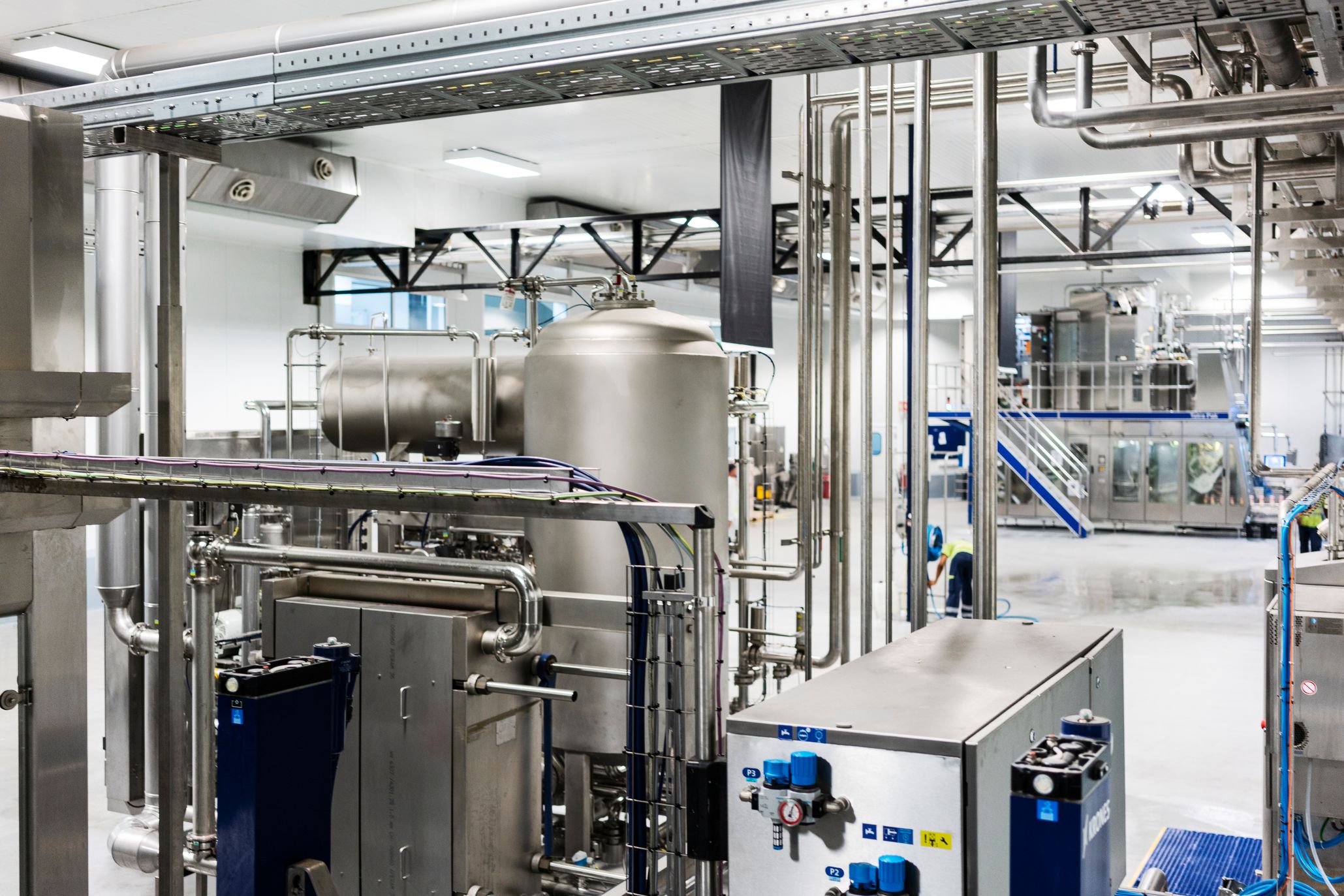
The plant in question for this case study was only 3 years old when CoolPlanet won the contract to deliver savings on this 8MW (cooling capacity) ammonia plant via a shared savings contract.

Key Stats

17%

Energy reduction

$0

Capex

0

Major equipment installed

We undertook the following activities:

• Building a full plant digital twin
• Modelling and understanding all cooling loads
• Recommissioning of the system,
• Developing enhanced controls and
• Plant analytics and optimisation via CoolPlanetOS
• Multiple small optimisation projects
• Full training of operators to deliver and maintain savings

By doing so we delivered 16% savings across 12 months (taking seasonality into account) to the customer via a shared savings, performance contract. All that without the customer spending any capex.

Challenges

The following are some of the issues which we typically see which are causing excessive energy consumption in meat factory refrigeration plants:

• Using simple energy KPI’s (kWh’s per tonne or kWh’s per head of cattle killed) that do not highlight either energy losses OR savings opportunities during dynamic conditions i.e. weather changes, production increases/ decreases or product mix changes
• No real understanding of how production changes (product mix changes for example) can drive energy consumption changes
• Insufficient automation in place or;
• Automation switched off (maybe initially only temporarily) and plants running in manual
• Plants do not dynamically adapt to changing weather and to production conditions
• Plant equipment consuming more power and water than design due to lack of maintenance or incorrect installation

Background

The plant was a very well designed plant with a top of the line SCADA system, inverters on most compressors, pumps and fans. However with 4 temperature profiles (ammonia, glycol, chilled water and typhoxic) levels and multiple product lines it is a complex plant.

The plant, while very high specification, was not fully commissioned and operator training wasn’t what it should have been. This is a typical situation in Industrial Refrigeration, where plants are deemed commissioned once they meet the temperature levels required – however they may be consuming 20 30% more power than necessary.

While the plant had a good SCADA system, and instrumentation generally, the operators made little use of the data available to review performance and optimise the plant. The plant was also statically controlled throughout the year i.e. not optimised to take into account changing weather conditions, production rates and product mixes.

Previously the customer had been monitoring plant performance using a kWh/T (of product) but this masked many issues in the plant. One of the issues was that as the breaded product dropped off the power consumption of the plant did not drop with it.

Breaded products came from a fryer at 80 deg C straight into a spiral freezer. Compared to say, burgers (at circa -2 deg C) the refrigeration load increase on the refrigeration system is significant. When the breaded product lines were reduced in favour of burgers (total tonnes stayed the same) the plant KPI (kWh/T) did not drop like it should have.

The reason?

There were significant operational issues with the plant that we shall discuss in detail below.

Pre-work: setting up for success

Understanding what was driving energy consumption

The first step was to understand the basics of what was driving energy consumption in the plant. As discussed above, the plant was quite complex with 5 different product lines requiring cooling at 4 different temperatures.

Energy consumption of refrigeration plants in meat processing plants are driven by a number of factors:

• Weather – mainly wet bulb temperature i.e. what is the ambient temperature and how humid is it
• Production rate i.e. head of cattle or pigs per day or number of birds
• Product mix i.e. more burgers or less burgers vs breaded products
• Maintenance status of the plant i.e. are the condensers fouled or full of air

As discussed the plant used a simple KPI (kWh of electricity per tonne of product) to track energy performance. These simple KPI’s are problematic however, as:

• They don’t account for reduced kill rates: if kill rate drops by 30% the refrigeration consumption will not drop by the same amount - the same production spaces need be the cooled at the same amount of workers work in the plant, also chilling tunnels may run at part load capacity, ie not as full as they had previously been but still need to be operational

• They don’t account for product mix - If the plant starts to produce less burgers (for example) the spiral freezers might be used less - however total plant tonnes might be stable because there is a corresponding increase in a product line that uses Low Temperature cooling.

As discussed these simple KPI’s were masking energy losses. A far more robust method of tracking energy consumption is to use statistical analysis tools. These tools take into account all the variables discussed above to generate models which can accurately predict what the overall refrigeration consumption will be when weather conditions or production varies.

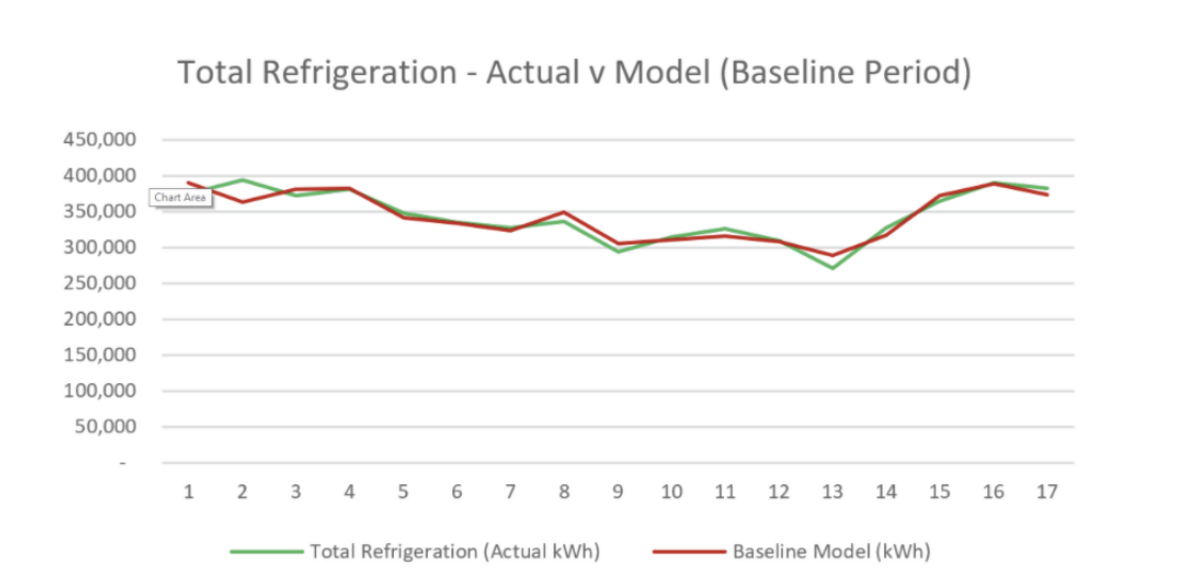
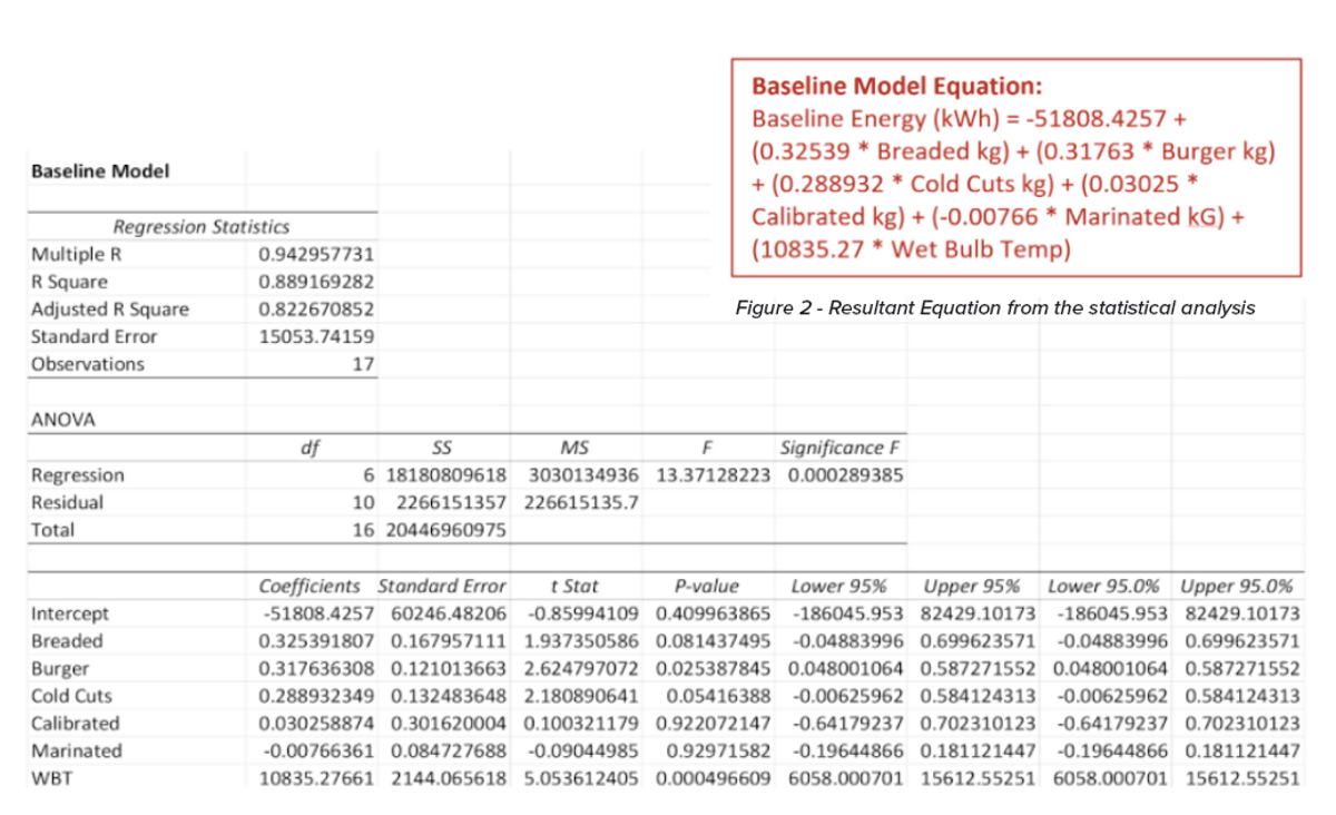
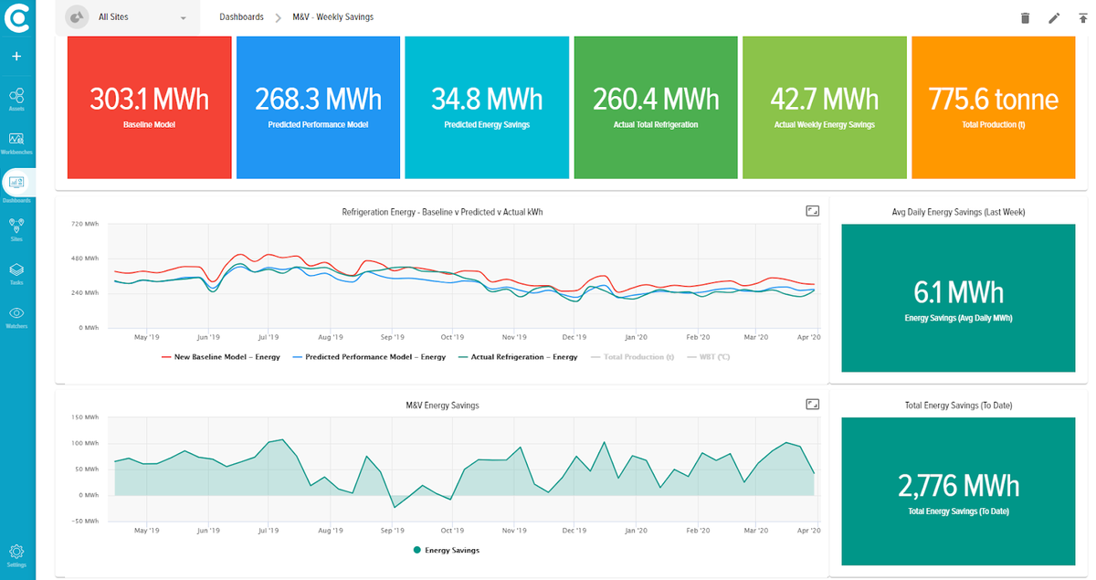
The statistical analysis fridge energy model is assessing weekly totals for each production line (breaded, burger, marinated etc.) along with average wet bulb temperature (WBT) to understand impact on total refrigeration energy use. A strong correlation between actual refrigeration and modelled refrigeration is shown in the chart over in figure 3.

In depth performance modelling of plant components

Cooling Loads

The first step was to understand the basics of what was driving energy consumption in the plant. As discussed above, the plant was quite complex with 5 different product lines requiring cooling at 4 different temperatures. The cooling loads are what drive the energy consumption of the plant. Plants have various loads at varying temperatures i.e.

• Production spaces - circa 46.4°F / 8°C

• Spiral Freezers -22°F / -30 °C

• Cold Stores -4°F / -20°C

• HVAC 71.6°F /+22 deg°C

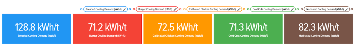
Further to the above, different products will have different cooling requirements entering a spiral freezer. For example a breaded product (chicken nugget) requires circa 80% more cooling than a burger for the same weight.

Being able to model that load and understand how product changes drive energy consumption in the plant delivers huge insights i.e. how is the plant performing versus the load that was actually on the plant.

Compressors

The motor power drawn by the compressor is a function of the work done in compressing the ammonia, and thus is a function of the incoming temperature pressure, ammonia flow rate, the discharge temperature and pressure, the slide valve position and the motor speed.

The 12 compressors were modelled and the performance of actual vs. predicted model output were compared. This allowed us to see for each individual machine how they should have performed vs actual with real world conditions.

This also allowed us to model target discharge pressure/temperature for the load on the plant and the ambient temperature (wet bulb). As can be seen below the target temperature (green) for the common discharge pressure is calculated by the model (based on condenser capacity, heat rejection and wet bulb) and compared with actual. As can be seen as we go from left to right (1 year) the green deviates from blue – indicating some scaling on the condensers (due to water treatment issues).

Condensors

We also built detailed models of the condensers taking the work done on cooling loads and compressors. By taking the heat rejection and prevailing ambient temperature we were able to develop a model which predicted the condenser power consumption and water use. This model was then used to dynamically compare the actual condenser water and power consumption with actual.

We used the CoolPlanet energy intelligence platform (CoolPlanetOS) to load these models into - from there we connected to the site SCADA system to pull in the live variables, which were used to populate the model. The model was then run dynamically and continuously to compare actual consumption with predicted (based on load, compressors operating and ambient).

As can be seen below the predicted consumption (green) was predicting significantly less condenser consumption than was actually (red) occurring at the left hand side of the graph.

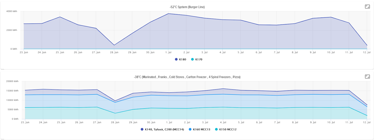
We investigated the issue and why the condensers and the high stage system energy had increased significantly. The system had a large volume of air that had been introduced into the system via one of the -61.6°F / -52°C system (-0.5 bar) compressors after a shaft seal had been allowing air to be introduced into the system. The automatic air purger on the system was unable to remove the air as the volume was too high. Multiple manual air purging was carried out and the results can be seen in the graph above. In addition to the condenser fan savings significant savings were achieved on the high stages of the system, the 21.2°F / -6 °C and 35.6°F / +2°C system.

Using the data to optimise

Bringing CoolPlanetOS to bear

We spent a lot of time at the start of the project building the high level and asset level models which gave us huge insight into the performance of the plant as follows:

• How the plant reacted to changing product mixes

• Maintenance issues in the plant

• Operational issues i.e.

• -36.4°F / -38°C system being cooled from the -61.6°F / -52°C separator when it could have been fed from the -36.4°F / -38°C system - operators opening connecting valves for transient issues and not closing the valve again

• Pump speeds being set too high for winter/low load conditions

• Sequencing of compressors – being done manually when automatisation capability was available The next step is to bring those models to life i.e. feed them with live pressure, temperature data from the plant and calculate dynamically and continuously the predicted plant performance – and compare it to the actual.

CoolPlanet have developed a powerful Cloud based tool to do exactly that. CoolPlanetOS can connect to your plant SCADA systems, meters and sensors and extract the data we need to run the models built previously.

Upgrading Site SCADA

As discussed the plant had a good SCADA system, connected to all the individual compressor controllers and with lots of data available. However the plant was basically run in part manual all the time. As a result the plant was completely static as per the design specification and was not optimised to react to changing weather conditions and product mix. In addition the operators would make changes to the plant (based on temporary production requests) and not change the plant back.

CoolPlanet spent significant time optimizing the control, including:

• Optimizing the discharge pressure control based on load and ambient - using the calculated target discharge condensing temperature and run the condenser fans to this target set point

• Compressor sequencing

• Suction pressure controlling - staggering suction pressure setpoints to optimise compressor sequencing

• Rebalancing loads across compressors and temperature levels

Optimising via small projects

The next step was to identify opportunities for further optimisation via small optimisation projects (further to the operational and maintenance improvements which have been discussed above).

Transferring Loads between Temperature Levels

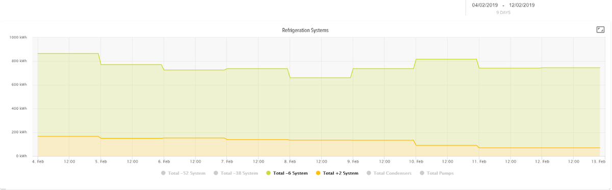
The models identified that the chilled water system load was high in comparison to the actual HVAC heat load for the internal corridors and offices. The chilled water temp was a fixed temperature all the year (irrespective of ambient conditions). The 42.8°F / -6°C glycol system was the largest system and was constantly in operation due to product freezing during production, the 42.8°F / -6°C system also serviced the chill stores and cold stores.

Having identified that the 35.6°F / 2°C system was overcooling for approximately 8 months of the year we modified the control of the system, this resulted in the system running at part load during the shoulder months. The system had previously run at part load and changing the control did yield significant savings. However we knew further savings could be achieved.

We modified the system to allow the chilled water system load to be transferred to the 42.8°F / -6°C system. In addition the temperature of chilled water was weather compensated to be based on ambient conditions. As can be seen below the load was taken off the 35.6°F / 2°C system and added to the 42.8°F / -6°C system (which had a much more optimally loaded compressor) – as can be see there was minimal impact on the 42.8°F / -6°C compressor power consumption.

Glycol Pump

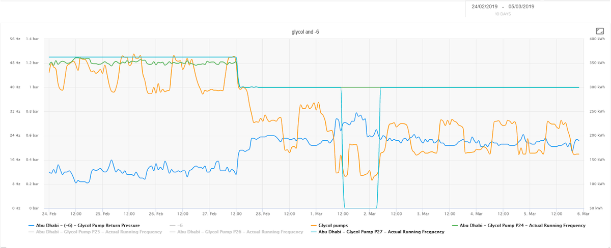
Our model and CoolPlanetOS highlighted that the Glycol system was not performing optimally - there appeared to be significant over-pumping in the glycol system as the return pressure was still very low. On further investigation it was discovered that parts of the Glycol system were not performing well and were being bypassed. We trialled lowering the pump speed and significant savings were achieved - circa 70kWe on average.

There were significant savings on the 42.8°F / -6°C compressors also.

Benefits

Through the range of solutions that we performed on the refrigeration plant the plant is now saving approximately $500k/yr. These savings are not only on the electrical load on the plant but on the reduction in water consumption.

The system now responds automatically to ambient conditions and production data without any manual intervention from the operators. The plant also gives the operators indicators and suggested causes of out of specification energy or water usage through our “watchers” system. The watchers system provides both alarm and reporting outputs to show where issues are occurring on the system pinpointing the likely causes and solutions which ensure that the savings are being maintained. The reporting requirements from the utilities department are now fully automatic and instant. This has greatly reduced the time consuming calculation and reporting for the onsite team.